def teta(z,tau,c): # c = 0 or 1
    c = np.double(c)/2
    n_max = 100.0 + c
    pi = np.pi
    t = 0.0 + 0.0j;
    for n in np.linspace(-n_max,n_max,2*n_max+1):
        t = t + np.exp(pi*1j* n*n*tau + 2*pi*n*1j*z)
    return t

def teta01(z,tau):
    t = teta(z+1.0/2,tau,0)
    return t


def teta11(z,tau):
    t = teta(z+1.0/2,tau,1)
    return t

def teta10(z,tau):
    t = teta(z,tau,1)
    return t

def teta00(z,tau):
    t = teta(z,tau,0)
    return t


def cn(u,k):
    # k -> tau
    # Reference: Wikipedia
    # https://ja.wikipedia.org/wiki/%E3%83%A4%E3%82%B3%E3%83%93%E3%81%AE%E6%A5%95%E5%86%86%E9%96%A2%E6%95%B0
    k_dash = np.sqrt(1.0 - k*k)
    l = 1.0/2 * (1.0 - np.sqrt(k_dash))/(1.0 + np.sqrt(k_dash))
    q = l + 2*np.power(l,5) + 15*np.power(l,9)  + 150*np.power(l,13) + 1707*np.power(l,17)
    tau = np.log(q) / (np.pi * 1j)
    # calculate
    t10 = teta10(0.0+0.0j , tau)
    t00 = teta00(0.0+0.0j , tau)
    t01 = teta01(0.0+0.0j, tau)
    # check print(np.sqrt(1.0 - np.power(t01/t00,4) )) = k
    z = u/(np.pi* t00 * t00)
    return t01 * teta10(z,tau) / (t10*teta01(z,tau))

Ke = sp.special.ellipk(1.0/2)
def schw_chrf(z):
    # reference: https://arxiv.org/pdf/1509.06344.pdf
    return (1.0 - 1.0j)/np.sqrt(2) * cn( Ke*(1.0+1.0j)/2 * z - Ke, 1.0/np.sqrt(2))
\begin{align} \vartheta(z,\tau) = \sum_{n=-\infty}^{\infty} \exp\left(\pi i n^2 \tau + 2\pi i n z \right) \end{align}
$q = \exp(\pi i \tau)$として
\begin{align} \vartheta_0(z,\tau) &:= \vartheta_{01}(z, \tau) = \sum_{n=-\infty}^{\infty} e^{\pi i \tau n^{2} + 2 \pi i n \left(z + \frac{1}{2}\right)} =1 + 2 \sum_{n=1}^{\infty} (-1)^{n} q^{n^{2}} \cos 2 n \pi z \end{align} \begin{align} \vartheta_{1}(z, \tau) &:= - \vartheta_{11}(z, \tau) = - \sum_{n=-\infty}^{\infty} e^{\pi i \tau \left(n + \frac{1}{2}\right)^{2} + 2 \pi i \left(n + \frac{1}{2}\right) \left(z + \frac{1}{2}\right)} =2\sum_{n=0}^{\infty}{(-1)^{n} q^{{\left(n + \frac{1}{2}\right)}^2} \sin(2 n + 1) \pi z} \end{align} \begin{align} \vartheta_{2}(z, \tau) &:= \vartheta_{10}(z, \tau) = \sum_{n=-\infty}^{\infty} e^{\pi i \tau \left(n + \frac{1}{2}\right)^2 + 2 \pi i \left(n + \frac{1}{2}\right)z} = 2 \sum_{n=0}^{\infty} q^{{\left(n+\frac{1}{2}\right)}^2} \cos (2 n + 1) \pi z \end{align} \begin{align} \vartheta_3(z, \tau) &:= \vartheta_{00}(z, \tau) = \sum_{n=-\infty}^{\infty} e^{i \pi \tau n^{2} + 2 \pi i n z} = 1 + 2 \sum_{n=1}^{\infty} q^{n^{2}} \cos 2 n \pi z. \end{align}
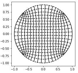
for x_i in x_m:
    z_h = x_i*np.ones(m) + x*1j
    z_v = x+1j*x_i*np.ones(m)
    w_h = schw_chrf(z_h)
    w_v = schw_chrf(z_v)
    plt.plot(np.real(w_h),np.imag(w_h),color='black')
    plt.plot(np.real(w_v),np.imag(w_v),color='black', linestyle='dashed')

plt.gca().set_aspect('equal', adjustable='box')

sc = 1.1
plt.xlim(-s*sc,s*sc)
plt.ylim(-s*sc,s*sc)
plt.show()
4. 画像への適用
今回用いるのは,このような将棋の画像です.
# load image
img = cv2.imread('picture_c/base200.png')
#img = cv2.cvtColor(img, cv2.COLOR_RGB2GRAY)

# show image with matplotlib
pix = img.shape[0]
x = np.linspace(-1,1,pix+1) # define square

plt.imshow(cv2.cvtColor(img, cv2.COLOR_BGR2RGB))
plt.gray()

# text mapping
# schwartz christoffel mapping
import sys

for i in range(pix):
    sys.stdout.write(str(i))
    sys.stdout.write(" ")
    for j in range(pix):
        tx_z = np.array([x[i],x[i+1],x[i+1],x[i]])
        ty_z = np.array([x[j],x[j],x[j+1],x[j+1]])
        zt = tx_z + 1j*ty_z
        w_h = schw_chrf(zt)
        tx = np.real(w_h)
        ty = np.imag(w_h)
        clr_b = np.double(img[ pix - j - 1 , i,0])/256
        clr_g = np.double(img[pix - j - 1 , i,1])/256
        clr_r = np.double(img[pix - j - 1 , i,2])/256
        plt.fill(tx,ty,color=(clr_r,clr_g,clr_b))

plt.gca().set_aspect('equal', adjustable='box')
sc = 1.1
plt.xlim(-s*sc,s*sc)
plt.ylim(-s*sc,s*sc)
plt.show()
plt.savefig("output/base.png")


 エルピクセル編集部