5. Update the parameters
Same as the Perceptron algorithm, logistic regression uses gradient descent optimization algorithm to update weights and biases. In order to do this, we need to calculate the derivative of cost function.
Derivative of sigmoid function:
$$\phi'(z)=\frac{\mathrm{d} }{\mathrm{d} z}(\frac{1}{1+e^{-z}})=\frac{e^{-z}}{(1+e^{-z})^2}=\frac{1+e^{-z}-1}{(1+e^{-z})^2}=\frac{1}{1+e^{-z}}-\frac{1}{(1+e^{-z})^2}=\phi(z)(1-\phi(z))$$
Derivative of cost function: J with respect to the activation $\phi(z)$ (denote this as "a"):
$$\frac{\partial J}{\partial a}=\frac{\partial }{\partial a}(-\frac{1}{m}\sum_{i=1}^{m}(y^{(i)}log(a)+(1-y^{(i)})log(1-a))=\frac{1-y}{1-a}-\frac{y}{a}$$
Derivative of cost function: J with respect to weights:
$$dw=\frac{\partial J}{\partial w}=\frac{\partial J}{\partial a}\frac{\partial a}{\partial z}\frac{\partial z}{\partial w}=\frac{1}{m}(\frac{1-y}{1-a}-\frac{y}{a})*a(1-a)*X.T$$
Derivative of cost function: J with respect to bias:
$$db=\frac{\partial J}{\partial b}=\frac{\partial J}{\partial a}\frac{\partial a}{\partial z}\frac{\partial z}{\partial b}=\frac{1}{m}np.sum((\frac{1-y}{1-a}-\frac{y}{a})*a(1-a))$$
Gradient descent algorithm:
$$weights=weights-learning\_rate*dw$$
$$bias=bias-learning\_rate*db$$
6. Repeat step 2-5 until the convergence of cost function
7. The complete logistic regression code
import numpy as np

class Logistic_regression:
    """Logistic regression classifier

    === Public Attributes ===
    learning_rate:
        A hyper-parameter that controls how much we are adjusting the weights
        of the network with respect the loss gradient.
    num_iterations:
        Number of iterations of the optimization loop.
    weight:
        This determines the strength of the connection of the neurons.
    bias:
        Bias neurons allow the output of an activation function to be shifted.
    """
    learning_rate: float
    num_iterations: int
    weight: np.array
    bias: np.array

    def __init__(self, learning_rate, num_iterations) -> None:
        """Initialize a new Logistic_regression with the provided
        <learning_rate> and <num_iterations>
        """
        self.learning_rate = learning_rate
        self.num_iterations = num_iterations
        self.weight = np.array([0])
        self.bias = np.array([0])

    def net_input(self, x: np.array) -> np.array:
        """Calculate the input of the activation function.

        :param x: input data, of shape (n_x, n_samples)
        :return: the input of the activation function
        """
        return np.dot(self.weight, x) + self.bias

    def predict(self, x: np.array) -> np.array:
        """Linear part -> Activation function (sigmoid).  Calculate the output prediction.

        :param x: input data, of shape (n_x, n_samples)
        :return: the output prediction
        """
        return self.sigmoid(self.net_input(x))

    def sigmoid(self, z: np.array) -> np.array:
        """Sigmoid function.

        :param x: input of the activation function: z
        :return: output of the sigmoid function
        """
        return 1/(1+np.exp(-z))

    def gradient(self, x: np.array, y: np.array, y_pred: np.array) -> tuple:
        """Calculate the gradients: dw and db

        :param x: input data, of shape (n_x, n_samples)
        :param y: true label vector, of shape (1, n_samples)
        :param y_pred: predicted label vector, of shape (1, n_samples)
        :return: derivatives of cost function: J with respect to weight: w and bias: b
        """
        m = x.shape[1]
        epsilon = 10**-8
        da = np.divide(1-y, 1-y_pred+epsilon) - np.divide(y, y_pred+epsilon)
        dz = da*self.sigmoid(self.net_input(x))*(1-self.sigmoid(self.net_input(x)))

        dw = np.dot(dz, x.T)/m
        db = np.sum(dz, axis=1, keepdims=True)/m
        return dw, db

    def fit(self, x: np.array, y: np.array) -> np.array:
        """Fit training data

        :param x: input data, of shape (n_x, n_samples)
        :param y: true label vector, of shape (1, n_samples)
        :return: the output prediction after training data
        """
        y_pred = np.array
        self.weight = np.random.randn(1, x.shape[0])*0.01
        self.bias = np.zeros((1, 1))

        for i in range(self.num_iterations):
            y_pred = self.predict(x)

            dw, db = self.gradient(x, y, y_pred)

            self.weight -= self.learning_rate*dw
            self.bias -= self.learning_rate*db

        return np.where(y_pred >= 0.5, 1, 0)
logistic_regression.py
Training the logistic regression model on the iris dataset
We are going to apply this logistic regression algorithm to the iris dataset, which is very similar to what we did with Perceptron algorithm (please refer to the previous article).
The iris dataset consists of:
- 150 samples
- 3 labels (species of iris): $setosa, virginica, versicolor$
- 4 features: $sepal\:length, sepal\:width, petal\:length, petal\:width (in\:cm)$
For this example, we will only use $setosa$ and $versicolor$ for labels, $sepal\:length$ and $petal\:length$ for features.
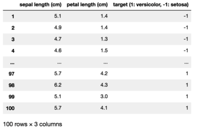
import pandas as pd
from sklearn import datasets

# acquire Data
iris = datasets.load_iris()
X = iris.data
y = iris.target

# select only "setosa" and "versicolor"
# extract only "sepal length" and "petal length"
X = np.delete(X, [1, 3], axis=1)
delete_target = np.where(y == 2)
y = np.delete(y, delete_target)
X = np.delete(X, delete_target, axis=0)
y = np.where(y == 0, -1, 1)

# visualize the data using Pandas DataFrame
pd.set_option('display.max_rows', 9)
pd.DataFrame({'sepal length (cm)': X[:, 0], 'petal length (cm)': X[:, 1],
              'target (1: versicolor, -1: setosa)': y},
              index=np.arange(1, len(X)+1))
iris_data.py
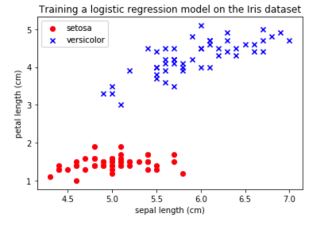
# plot data
setosa = np.where(y == 0)
versicolor = np.where(y == 1)
plt.scatter(X[setosa, 0], X[setosa, 1],
            color='red', marker='o', label='setosa')
plt.scatter(X[versicolor, 0], X[versicolor, 1],
            color='blue', marker='x', label='versicolor')
plt.title('Training a logistic regression model on the Iris dataset')
plt.xlabel('sepal length (cm)')
plt.ylabel('petal length (cm)')
plt.legend(loc='upper left')
plt.show()
iris_data.py
Now, we will create a $Logistic\_regression$ object by setting the learning rate and number of iterations. Then, train the perceptron model by calling $fit$ method with two arguments: input data and true label vector.
# training the logistic regression model
logit_model = Logistic_regression(learning_rate=0.1, num_iterations=100)
y_pred = logit_model.fit(X.T, y.reshape(1, -1))  #change y shape from (100, ) to (1, 100)
train_data.py
The result can be visualized by plotting the decision boundary and data. Again, we will use matplotlib to show data with boundary line which was trained by the model.
# plot the decision boundary and data
x_ax = np.arange(X[:, 0].min()-1, X[:, 0].max()+1, 0.01)
w1 = logit_model.weight[:, 0]
w2 = logit_model.weight[:, 1]
b = logit_model.bias[0]
plt.plot(x_ax, -w1*x_ax/w2 - b/w2, color='black')

setosa = np.where(y == 0)
versicolor = np.where(y == 1)
plt.scatter(X[setosa, 0], X[setosa, 1],
            color='red', marker='o', label='setosa')
plt.scatter(X[versicolor, 0], X[versicolor, 1],
            color='blue', marker='x', label='versicolor')
plt.title('Training a logistic regression model on the Iris dataset')
plt.xlabel('sepal length (cm)')
plt.ylabel('petal length (cm)')
plt.legend(loc='upper left')
plt.show()

print('Accuracy: ' + str(np.mean(y_pred == y) * 100) + '%')
visualize_result.py
 Shion Fujimori