Machine Learning with Python Part.1 ~Perceptron~

import numpy as np

class Perceptron:
    """Perceptron classifier

    === Public Attributes ===
    learning_rate:
        A hyper-parameter that controls how much we are adjusting the weights
        of the network with respect the loss gradient.
    num_iterations:
        Number of iterations of the optimization loop.
    weight:
        This determines the strength of the connection of the neurons.
    bias:
        Bias neurons allow the output of an activation funcrtion to be shifted.
    """
    learning_rate: float
    num_iterations: int
    weight: np.array
    bias: np.array

    def __init__(self, learning_rate, num_iterations) -> None:
        """Initialize a new Perceptron with the provided
        <learning_rate> and <num_iterations>
        """
        self.learning_rate = learning_rate
        self.num_iterations = num_iterations
        self.weight = np.array([0])
        self.bias = np.array([0])

    def net_input(self, x: np.array) -> np.array:
        """Calculate the input of the activation function

        :param x: input data, of shape (n_x, n_samples)
        :return: the input of the activation function
        """
        return np.dot(self.weight.T, x) + self.bias

    def predict(self, x: np.array) -> np.array:
        """Activation function.  Calculate the output prediction

        :param x: input data, of shape (n_x, n_samples)
        :return: the output prediction
        """
        return np.where(self.net_input(x) > 0, 1, -1)

    def fit(self, x: np.array, y: np.array) -> np.array:
        """Fit training data

        :param x: input data, of shape (n_x, n_samples)
        :param y: true label vector, of shape (1, n_samples)
        :return: the output prediction after training data
        """
        m = x.shape[1]
        y_pred = np.array
        self.weight = np.random.randn(x.shape[0], 1)*0.01
        self.bias = np.zeros((1, 1))

        for i in range(self.num_iterations):
            y_pred = self.predict(x)

            dw = (1/m)*np.dot(x, (y_pred-y).T)
            db = (1/m)*np.sum(y_pred-y)

            self.weight -= self.learning_rate*dw
            self.bias -= self.learning_rate*db

        return y_pred

perceptron.py

Training the Perceptron model on the iris dataset

The purpose of this example is to create the model that can classify the different species of the iris flower. Scikit-learn, a free software machine learning library for Python, has a inbuilt datasets for the iris classification problem.

The dataset consists of:
- 150 samples
- 3 labels (species of iris): $setosa, virginica, versicolor$
- 4 features: $sepal\:length, sepal\:width, petal\:length, petal\:width (in\:cm)$

For this example, we will only use $setosa$ and $versicolor$ for labels, $sepal\:length$ and $petal\:length$ for features.

from sklearn import datasets

# acquire Data
iris = datasets.load_iris()
X = iris.data
y = iris.target

# select only "setosa" and "versicolor"
# extract only "sepal length" and "petal length"
X = np.delete(X, [1, 3], axis=1)
delete_target = np.where(y == 2)
y = np.delete(y, delete_target)
X = np.delete(X, delete_target, axis=0)
y = np.where(y == 0, -1, 1)

iris_data.py

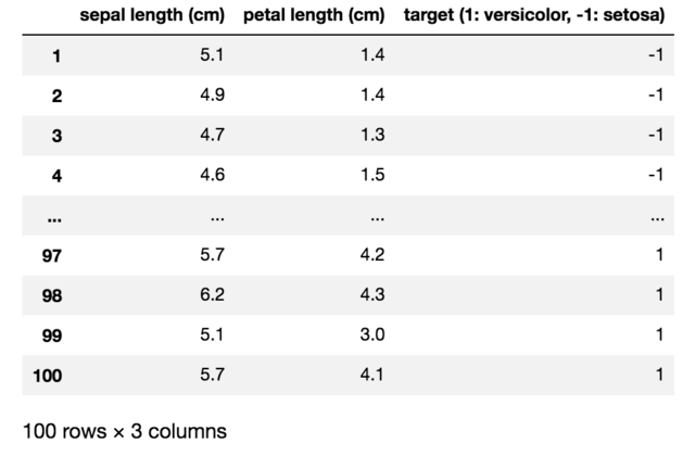
We will use Pandas DataFrame to visualize the data.

import pandas as pd

pd.set_option('display.max_rows', 9)
pd.DataFrame({'sepal length (cm)': X[:, 0], 'petal length (cm)': X[:, 1], 
              'target (1: versicolor, -1: setosa)': y}, 
              index=np.arange(1, len(X)+1))

visualize_data.py

Also, we will use Matplotlib, a Python 2D plotting library, to show a graph of iris dataset.

import matplotlib.pyplot as plt

setosa = np.where(y == -1)
versicolor = np.where(y == 1)
plt.scatter(X[setosa, 0], X[setosa, 1],
            color='red', marker='o', label='setosa')
plt.scatter(X[versicolor, 0], X[versicolor, 1],
            color='blue', marker='x', label='versicolor')
plt.title('Training a perceptron model on the Iris dataset')
plt.xlabel('sepal length (cm)')
plt.ylabel('petal length (cm)')
plt.legend(loc='upper left')
plt.show()

visualize_data.py

Now, we will create a $Perceptron$ object by setting the learning rate and number of iterations. Then, train the perceptron model by calling $fit$ method with two arguments: input data and true label vector.

ppn = Perceptron(learning_rate=0.3, num_iterations=10)
y_pred = ppn.fit(X.T, y)

train_data.py

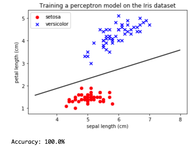
The result can be visualized by plotting the decision boundary and data. Again, we will use Matplotlib to show data with boundary line which was trained by the model.

x_ax = np.arange(X[:, 0].min()-1, X[:, 0].max()+1, 0.01)
w1 = ppn.weight[0]
w2 = ppn.weight[1]
b = ppn.bias[0]
plt.plot(x_ax, -w1*x_ax/w2 - b/w2, color='black')

setosa = np.where(y == -1)
versicolor = np.where(y == 1)
plt.scatter(X[setosa, 0], X[setosa, 1],
            color='red', marker='o', label='setosa')
plt.scatter(X[versicolor, 0], X[versicolor, 1],
            color='blue', marker='x', label='versicolor')
plt.title('Training a perceptron model on the Iris dataset')
plt.xlabel('sepal length (cm)')
plt.ylabel('petal length (cm)')
plt.legend(loc='upper left')
plt.show()

print('Accuracy: ' + str(np.mean(y_pred == y) * 100) + '%')